Difference between revisions of "Discussion7S16"
(→Raycast: Initial draft.) |
(→Overview: Added week 7.5 discussion slides.) |
||
| (3 intermediate revisions by one user not shown) | |||
| Line 3: | Line 3: | ||
Slides: [http://ivl.calit2.net/wiki/images/2/25/Week_7_DiscussionS16.pdf Download here] | Slides: [http://ivl.calit2.net/wiki/images/2/25/Week_7_DiscussionS16.pdf Download here] | ||
| + | |||
| + | Week 7.5 Discussion, from lecture(05/12/16) | ||
| + | |||
| + | Slides: [http://ivl.calit2.net/wiki/images/b/bf/Week_7.5_Discussion.pdf Download here] | ||
==Bezier Curves== | ==Bezier Curves== | ||
| + | The idea of Bezier curves(or any spline curve really) is that we specify a small set of control points, and interpolate between them to find a continuous curve. | ||
| + | |||
| + | Bezier curves are exceptionally useful, and are used heavily in rendering and animation, due to how easily controllable they are. But they can be a bit mysterious, especially if math isn't your forte (After all, we are taking a handful of discrete points and creating a continuous curve from them!). So we've put together a short explanation on how Bezier curves work: starting from the mathematical point of view and ending with a simple implementation. | ||
| + | |||
| + | ===The General Form=== | ||
| + | The general form of a Bezier curve can have any number of control points. | ||
| + | |||
| + | [[File:Bezier00.PNG|500px]] | ||
| + | |||
| + | Here ''q'' is the point along the curve at time ''t'' we are trying to evaluate. ''n'' is the number of control points, and each ''i'' represents which control point we're on. If we find a sufficient number of ''q''s we can make a smooth enough curve, so being able to evaluate this equation quickly is key. In general, the more control points(higher ''n'') used to generate a curve, the more accurately it can represent various non-polynomial curves. | ||
| + | |||
| + | But there is a fairly massive diminishing return in the computing world: the amount of accuracy gained from each additional control point is terribly small in comparison to the increase in compute time needed to evaluate the curve. | ||
| + | |||
| + | ===The Cubic Bezier Form=== | ||
| + | So we make a compromise: use 4 control points and hope for the best! This is known as the Cubic Bezier curve due to ''n'' being 3. | ||
| + | |||
| + | Starting with 4 control points (''p_0'',''p_1'',''p_2'',''p_3''), and a time ''t'', we can interpolate all of the control points at time ''t'' using this equation: | ||
| + | |||
| + | [[File:Bezier01.PNG|500px]] | ||
| + | |||
| + | The the 3Ci combination expands to: | ||
| + | |||
| + | [[File:Bezier02.PNG|400px]] | ||
| + | |||
| + | where n! is n-factorial and is the product of the given number and all natural numbers less than it, for example, 3!=3∗2∗1. Note that this is going to be the same for each ''p'', as each ''i'' is staying constant. (Hint: Don't write a factorial function! This equation evaluates to a very predictable value always.) | ||
| + | |||
| + | |||
| + | At this point we notice that given some time t that the leading coefficient evaluates to a constant scalar, so we can replace it with a convenient function Ci(t): | ||
| + | |||
| + | [[File:Bezier03.PNG|500px]] | ||
| + | |||
| + | Which if we substitute into our cubic Bezier curve equations we get: | ||
| + | |||
| + | [[File:Bezier04.PNG|650px]] | ||
| + | |||
| + | ===The (mind-blowing) Matrix Form=== | ||
| + | The equation we just saw above is nothing more than adding together 4 vectors that have each been multiplied by a scalar weight! | ||
| + | |||
| + | [[File:Bezier05.PNG|700px]] | ||
| + | |||
| + | Pretty neat right? Well what's even more neat is that this is a matrix-vector product in disguise! | ||
| + | |||
| + | [[File:Bezier06.PNG|650px]] | ||
| + | |||
| + | |||
| + | So there you have it! We started with what seemed to be a complex sum and reduced it into a single matrix multiplication. Now you can very quickly find each ''q'' along the curve for many many ''t''s. | ||
| + | |||
| + | As an aside, this method of taking sums and forming a matrix multiplication out of them is a common method in Computer Graphics as matrix multiplication is exactly what the graphics hardware is optimized to do. | ||
==Selection Buffers== | ==Selection Buffers== | ||
| Line 31: | Line 83: | ||
So how do we implement this in OpenGL? Well, we first need the subroutine to redraw the selection buffer. Let's implement a method <code>selectionDraw</code> that draws the object, but with the selection shader instead. The ID is going to be remembered per selectable object we create. This ID will then be sent to our selection shader, which simply colors the whole object with a flat color based on that ID. | So how do we implement this in OpenGL? Well, we first need the subroutine to redraw the selection buffer. Let's implement a method <code>selectionDraw</code> that draws the object, but with the selection shader instead. The ID is going to be remembered per selectable object we create. This ID will then be sent to our selection shader, which simply colors the whole object with a flat color based on that ID. | ||
| − | [[File:Selectionbuffercode00.PNG| | + | [[File:Selectionbuffercode00.PNG|800px]] |
What about the Vertex shader you ask? Well we're drawing the object the same way that it's normally drawn in our display buffer. What should our vertex shader be then? | What about the Vertex shader you ask? Well we're drawing the object the same way that it's normally drawn in our display buffer. What should our vertex shader be then? | ||
| Line 39: | Line 91: | ||
Now all we need is some basic type conversion and we're good! | Now all we need is some basic type conversion and we're good! | ||
| − | [[File:Selectionbuffercode01.PNG| | + | [[File:Selectionbuffercode01.PNG|800px]] |
So we've gotten the object that we've selected. How do we now move that selection? Well that will be left as an exercise for the reader. :) | So we've gotten the object that we've selected. How do we now move that selection? Well that will be left as an exercise for the reader. :) | ||
Latest revision as of 20:36, 13 May 2016
Contents |
Overview
Week 7 Discussion recap(05/09/16)
Slides: Download here
Week 7.5 Discussion, from lecture(05/12/16)
Slides: Download here
Bezier Curves
The idea of Bezier curves(or any spline curve really) is that we specify a small set of control points, and interpolate between them to find a continuous curve.
Bezier curves are exceptionally useful, and are used heavily in rendering and animation, due to how easily controllable they are. But they can be a bit mysterious, especially if math isn't your forte (After all, we are taking a handful of discrete points and creating a continuous curve from them!). So we've put together a short explanation on how Bezier curves work: starting from the mathematical point of view and ending with a simple implementation.
The General Form
The general form of a Bezier curve can have any number of control points.
Here q is the point along the curve at time t we are trying to evaluate. n is the number of control points, and each i represents which control point we're on. If we find a sufficient number of qs we can make a smooth enough curve, so being able to evaluate this equation quickly is key. In general, the more control points(higher n) used to generate a curve, the more accurately it can represent various non-polynomial curves.
But there is a fairly massive diminishing return in the computing world: the amount of accuracy gained from each additional control point is terribly small in comparison to the increase in compute time needed to evaluate the curve.
The Cubic Bezier Form
So we make a compromise: use 4 control points and hope for the best! This is known as the Cubic Bezier curve due to n being 3.
Starting with 4 control points (p_0,p_1,p_2,p_3), and a time t, we can interpolate all of the control points at time t using this equation:
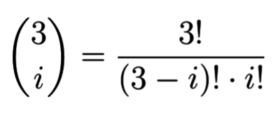
The the 3Ci combination expands to:
where n! is n-factorial and is the product of the given number and all natural numbers less than it, for example, 3!=3∗2∗1. Note that this is going to be the same for each p, as each i is staying constant. (Hint: Don't write a factorial function! This equation evaluates to a very predictable value always.)
At this point we notice that given some time t that the leading coefficient evaluates to a constant scalar, so we can replace it with a convenient function Ci(t):
Which if we substitute into our cubic Bezier curve equations we get:
The (mind-blowing) Matrix Form
The equation we just saw above is nothing more than adding together 4 vectors that have each been multiplied by a scalar weight!
Pretty neat right? Well what's even more neat is that this is a matrix-vector product in disguise!
So there you have it! We started with what seemed to be a complex sum and reduced it into a single matrix multiplication. Now you can very quickly find each q along the curve for many many ts.
As an aside, this method of taking sums and forming a matrix multiplication out of them is a common method in Computer Graphics as matrix multiplication is exactly what the graphics hardware is optimized to do.
Selection Buffers
Have you ever wondered how those light gun controllers for arcade games or console games worked? In Nintendo's game Duck Hunt, for example, the player points the light gun at a duck and push the trigger, and the game somehow registers that you hit the duck! The hint is in the fact that the name gun is actually a red herring.
The moment the player pushes the trigger, what happens is the whole image is redrawn—faster than the human eye can catch. This special re-render essentially draws all the shootable objects(e.g. ducks for Duck Hunt) in white, but everything else in black. Then, the light gun—equipped with a photodiode sensor—reads the specially redrawn image and senses whether the player pointed at a white portion or not, meaning the "gun" is actually more like a camera, and receives light instead of shooting light. (Read more here and here)
Borrowing Old Ideas
For doing selection in 3D, we can use a similar idea. When a user clicks, we redraw the whole scene with a special render, coloring each selectable object with a unique color.
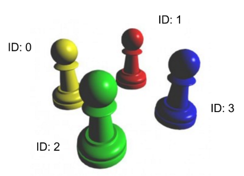
In order to do this, first we need to assign each object a unique ID that identifies what we've just selected. Let's look at the following chess pieces, and the following assigned IDs:
Now after we render this, we want to be able to retrieve the ID of each object back from the render. How might we accomplish that?
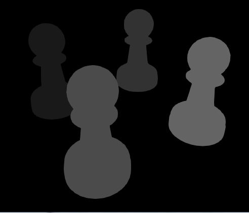
Well one way to do it would be to directly use the ID as the color! So ID 0 will be the darkest, and ID 3 will be the brightest object in this render. For example:
Great! Now when the user had clicked object 3 for example, they can read that pixel, see what the brightness is, and try to find out what object's color that matches to!
The grayscale image up there is the Selection Buffer rendering. In that particular selection buffer, we've exaggerated the differences between each of the objects. In a more typical setting you might use the color vec4(id/255.0f, 0.0f, 0.0f, 1.0f), meaning that each of those objects will actually be quite close in color.
The Code
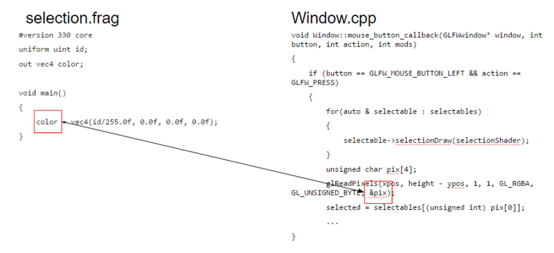
So how do we implement this in OpenGL? Well, we first need the subroutine to redraw the selection buffer. Let's implement a method selectionDraw that draws the object, but with the selection shader instead. The ID is going to be remembered per selectable object we create. This ID will then be sent to our selection shader, which simply colors the whole object with a flat color based on that ID.
What about the Vertex shader you ask? Well we're drawing the object the same way that it's normally drawn in our display buffer. What should our vertex shader be then?
Now let's handle the case when we actually call all the selectionDraws. This will happen on mouse click so we'd place it in our Window class's mouse_button_callback. On a left-button click, we draw every selectable object with the selectionShader, and then call glReadPixels to get the pixel value of where the user clicked. If we clicked an actual selectable, we're in essence retrieving the color that the selection.frag shader colored our object with.
Now all we need is some basic type conversion and we're good!
So we've gotten the object that we've selected. How do we now move that selection? Well that will be left as an exercise for the reader. :)
You can read more on this in the Lighthouse 3D-Picking Tutorial
Raycast
Raycasting is an alternate method for selection, done by determining where in 3D space our mouse clicked. Because our mouse works along a 2D x-y plane, but our world is in 3D, we need to convert from a 2D coordinate system to 3D. Does this sound familiar at all?
Hopefully it does, as it's basically the rasterization equation from the beginning of the quarter! Now of course, we aren't going from a point in 2D to a point in 3D here. Because we're going from a lower dimension to a higher dimension(2→3), we simply don't have enough information. So we decide that we're selecting everything along the Z-axis, or put in another way we're shooting a ray along the Z-axis, and hoping that it hits something.
By the way, we're simply going to go over an overview of this method in the context of this class, as this involves a bit more math than we want to add onto your Bezier curve calculations.
So raycasting goes like this:
- First shoot a ray from the camera towards the mouse pointer.
- Find the first object that intersects with that ray.
- That object is our selection.
It's really a beautifully simple way of determining object selection. The architecture is going to be a lot simpler than programming a selection buffer algorithm. Of course it involves a bit of intersection math(which usually becomes the bottleneck), but when you have 3D pointer devices(e.g. Nintendo Wiimote or Sony Move) this is definitely the more natural way of selecting objects than a selection buffer. However, modern graphics cards are so heavily optimized to deal with buffers, but less so with intersection(though that is changing with hardware ray tracing libraries such as Nvidia Optix) that sometimes the complicated architecture is worth it.
All in all, both selection methods have pros and cons that make them equally viable choices for selection.
If you want to learn more about ray casting, we recommend you read these excellently illustrated Ray Casting Notes or take CSE168, in which you'll learn Raytracing, where the math for rays are used everywhere.


